Member-By-Member postprocessor module
This module contains Data postprocessors classes applying the postprocessing algorithm detailed in
Bert Van Schaeybroeck and Stéphane Vannitsem. Ensemble post-processing using member-by-member approaches: theoretical aspects. Quarterly Journal of the Royal Meteorological Society, 141 (688):807–818, 2015. URL: https://doi.org/10.1002/qj.2397.
Basically, it corrects a provided Data object \(\mathcal{D}_{p,n,m,v} (t)\) provided by applying the formula:
where \(P\) is the total number of predictors (given by the attribute number_of_predictors of \(\mathcal{D}\)).
In the formula above:
The Data object \(\mathcal{D}_{p,n,m,v} (t)\) is assumed to contain all the predictors used to correct the variable needed, the first predictor being by convention the variable itself: \(\mathcal{D}_{0,n,m,v} (t)\).
\(\mu^{\rm ens}_{p,n,v} (t)\) is the
Data.ensemble_meanof the Data object \(\mathcal{D}_{p,n,m,v} (t)\).\(\tau_{v} (t)\) is a multiplicative correction applied to each member of the first predictor of the
Data.centered_ensemble\(\bar{\mathcal{D}}^{\rm ens}_{0,n,m,v} (t)\).\(\mathcal{D}^C_{n,m,v} (t)\) is the corrected Data object, with an ensemble member-by-member correction.
Content
Several different postprocessors are available, with different strategy to determine the coefficients \(\alpha_{v} (t)\), \(\beta_{p,v} (t)\) and \(\tau_{v}\):
BiasCorrection: A simple correction of the bias.EnsembleMeanCorrection: A correction of the ensemble mean.EnsembleSpreadScalingCorrection: A correction of the ensemble mean and a correction of the ensemble spread through a multiplicative scaling.EnsembleSpreadScalingAbsCRPSCorrection: A correction of the ensemble mean and a correction of the ensemble spread, with a tuning of the parameters to minimize the Absolute norm CRPS scoreData.Abs_CRPS().EnsembleSpreadScalingNgrCRPSCorrection: A correction of the ensemble mean and a correction of the ensemble spread, with a tuning of the parameters to minimize the Non-homogeneous Gaussian Regression (NGR) CRPS scoreData.Ngr_CRPS().EnsembleAbsCRPSCorrection: A correction of the ensemble mean and a correction of the ensemble spread with spread scaling and nudging. In addition, the parameters are tuned to minimize the Absolute norm CRPS scoreData.Abs_CRPS().EnsembleNgrCRPSCorrection: A correction of the ensemble mean and a correction of the ensemble spread with spread scaling and nudging. In addition, the parameters are tuned to minimize the Non-homogeneous Gaussian Regression (NGR) CRPS scoreData.Ngr_CRPS().
Postprocessors
We now detail these postprocessors:
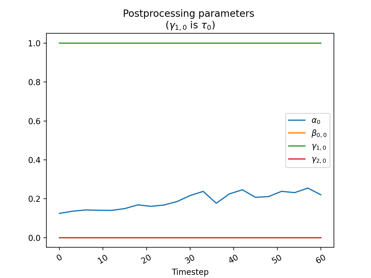
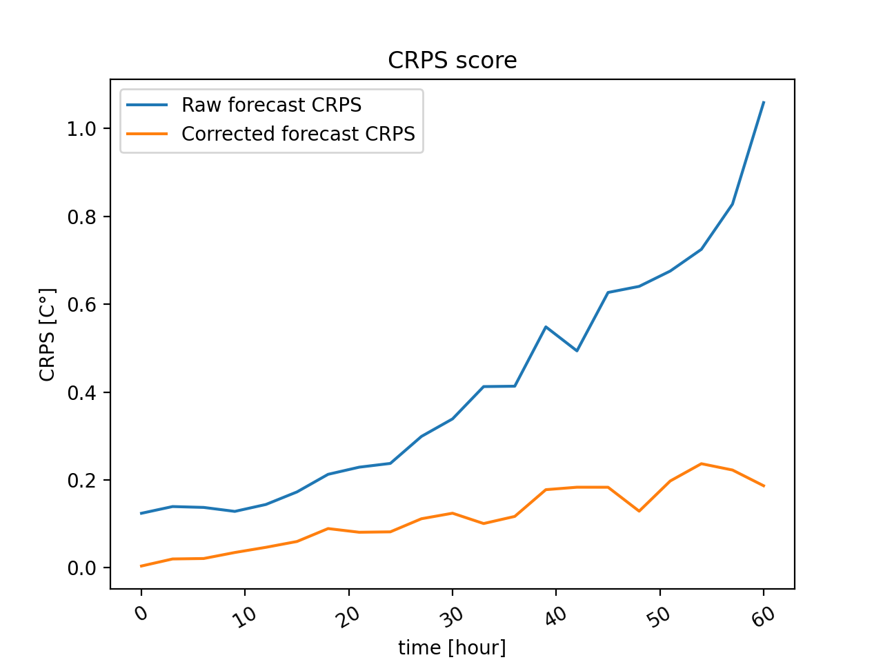
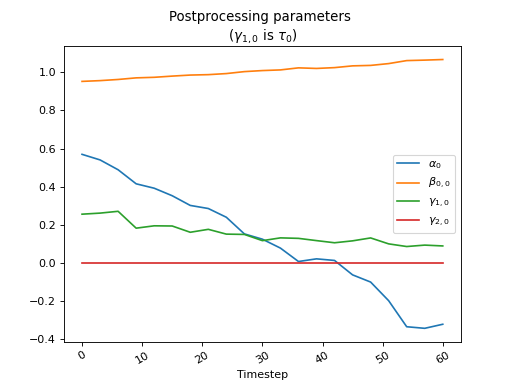
- class postprocessors.MBM.BiasCorrection[source]
Bases:
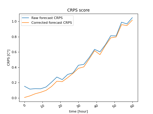
postprocessors.MBM.EnsembleMeanCorrectionA postprocessor to correct the bias. Correct according to the formula:
\[\mathcal{D}^C_{n,m,v} (t) = \alpha_{v} (t) + \sum_{p=1}^P \beta_{p,v} (t) \mu^{\rm ens}_{p,n,v} (t) + \tau_{v} (t) \bar{\mathcal{D}}^{\rm ens}_{0,n,m,v} (t)\]where \(\alpha_{v} (t) = \left\langle \mathcal{O}_{n,v} (t) - \mu^{\rm ens}_{0,n,v} (t) \right\rangle_n\) with \(\mathcal{O}_{n,v} (t)\) is the observation training set and \(\mu^{\rm ens}_{0,n,v} (t)\) is the ensemble mean of the first predictor of the training set, i.e. the
ensemble_meanof the predictor to correct. \(\bar{\mathcal{D}}^{\rm ens}_{0,n,m,v} (t)\) is thecentered_ensembleof the first predictor. We have also\(\beta_{0,v} (t) = 1\)
\(\beta_{p>0,v} (t) = 0\)
\(\tau_{v} (t) = 1\)
for all \(v\) and \(t\).
- parameters_list
The list of training parameters \(\alpha_{v} (t)\), \(\beta_{n,v} (t)\), \(\tau_{v} (t)\), as
Dataobjects. This list is empty until the firsttrain()method call.
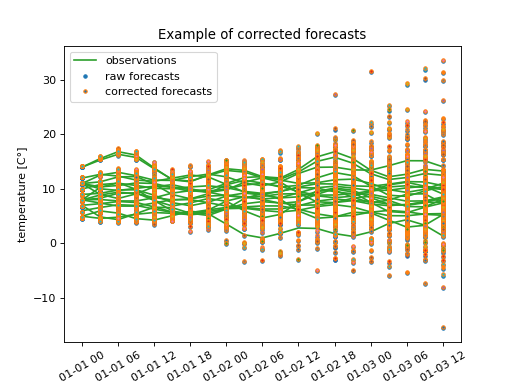
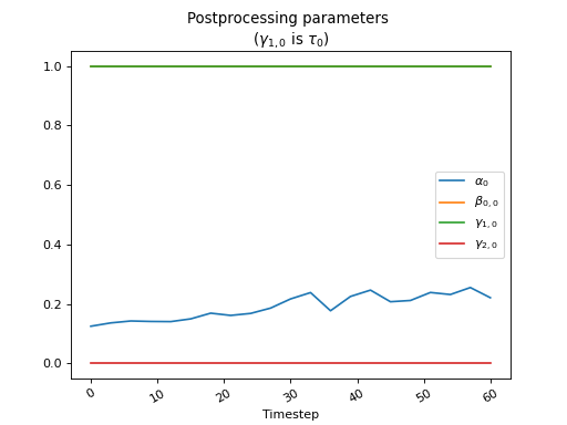
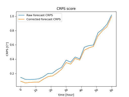
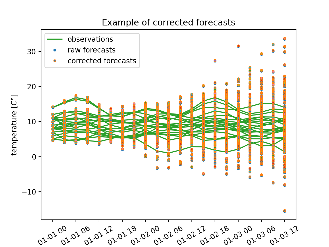
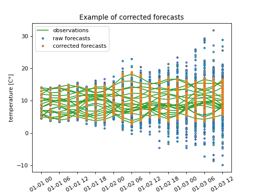
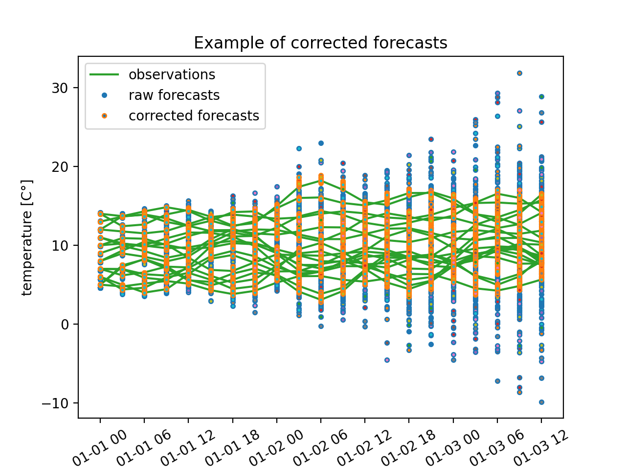
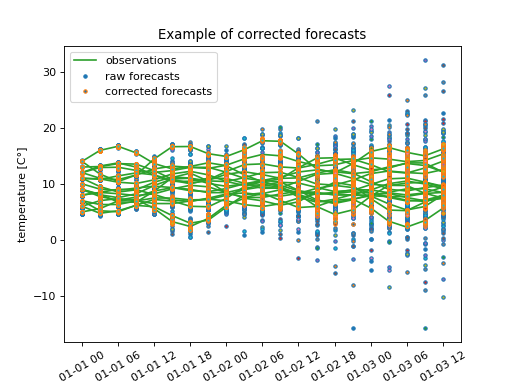
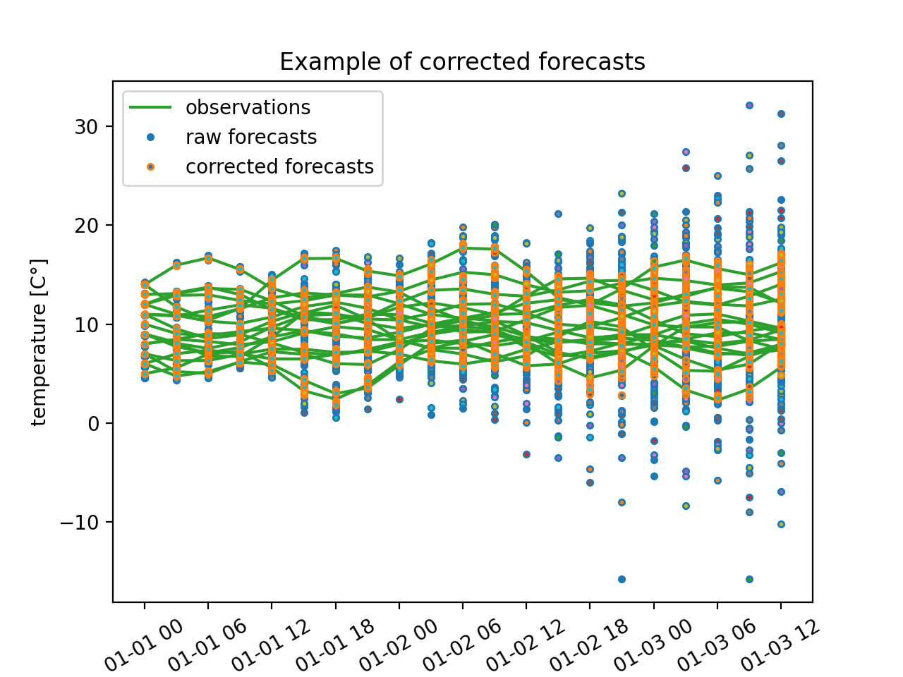
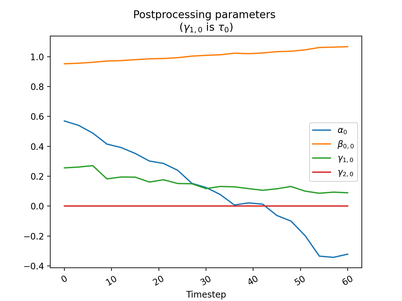
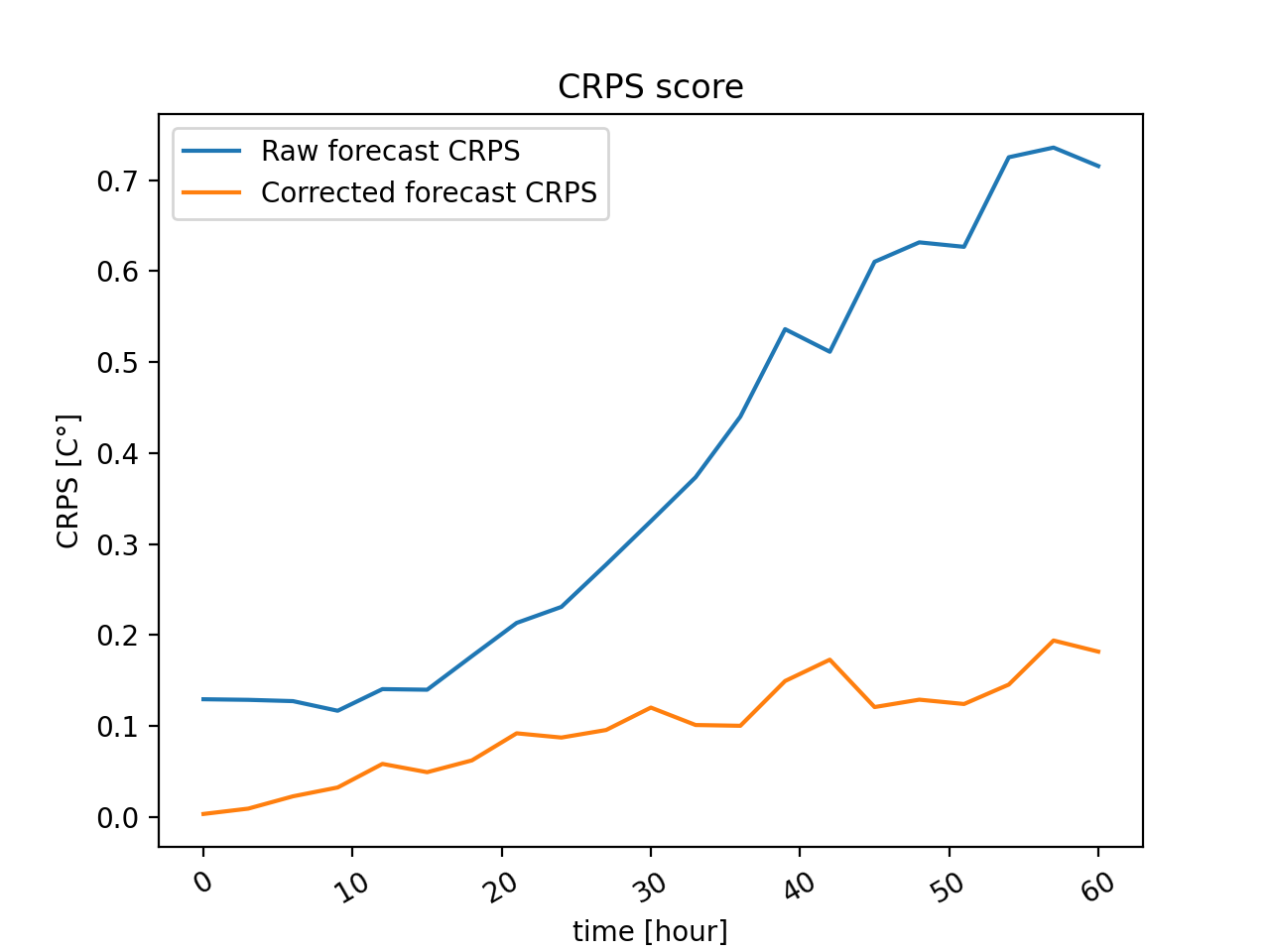
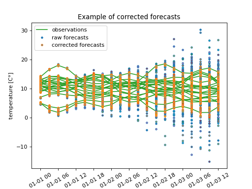
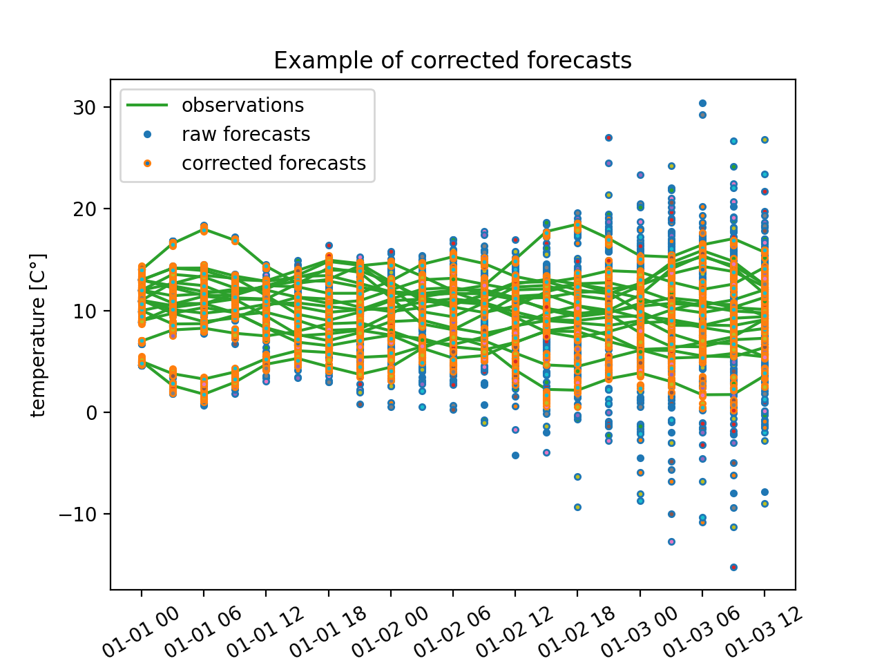
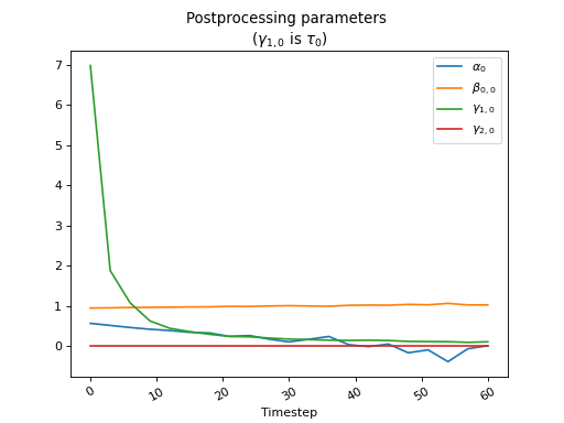
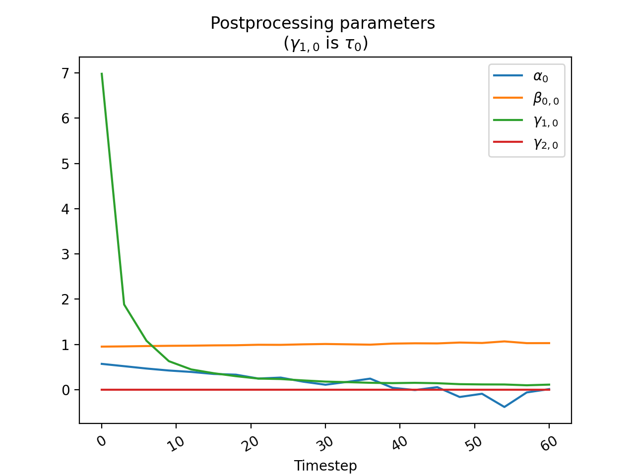
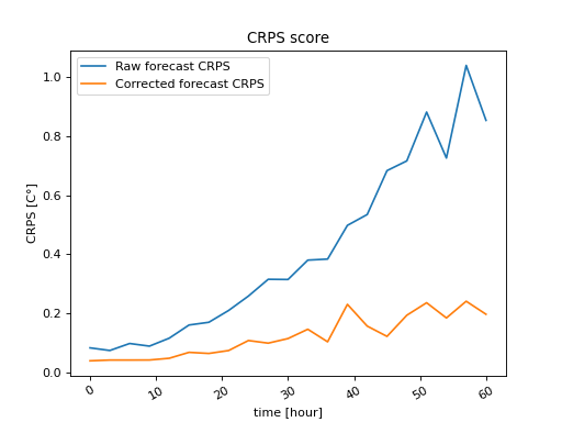
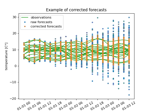
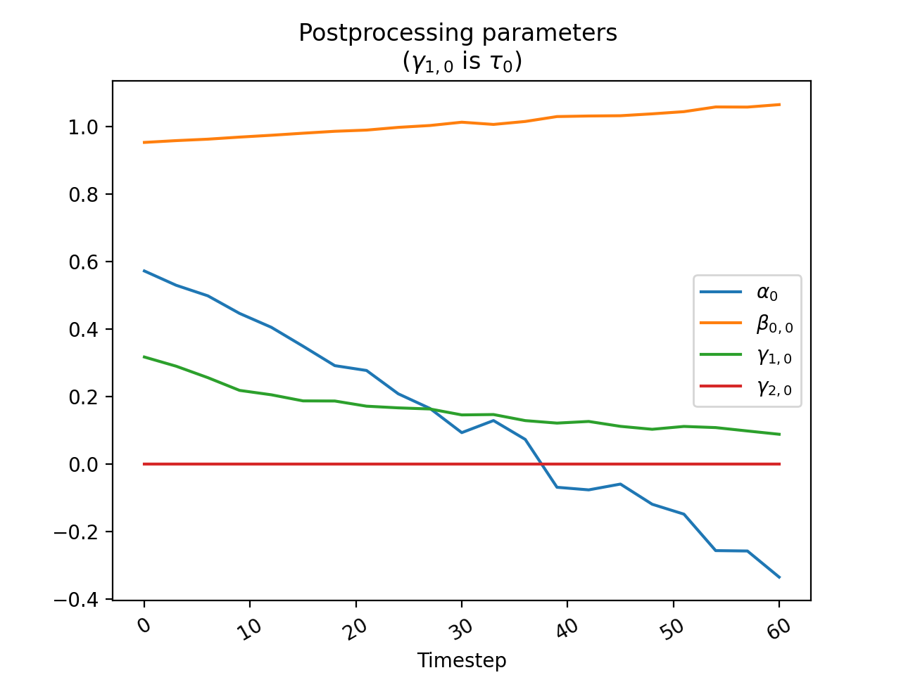
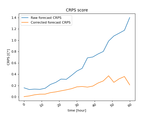
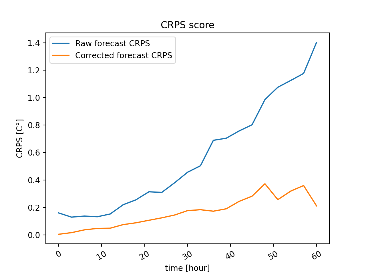
Examples
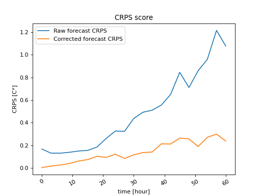
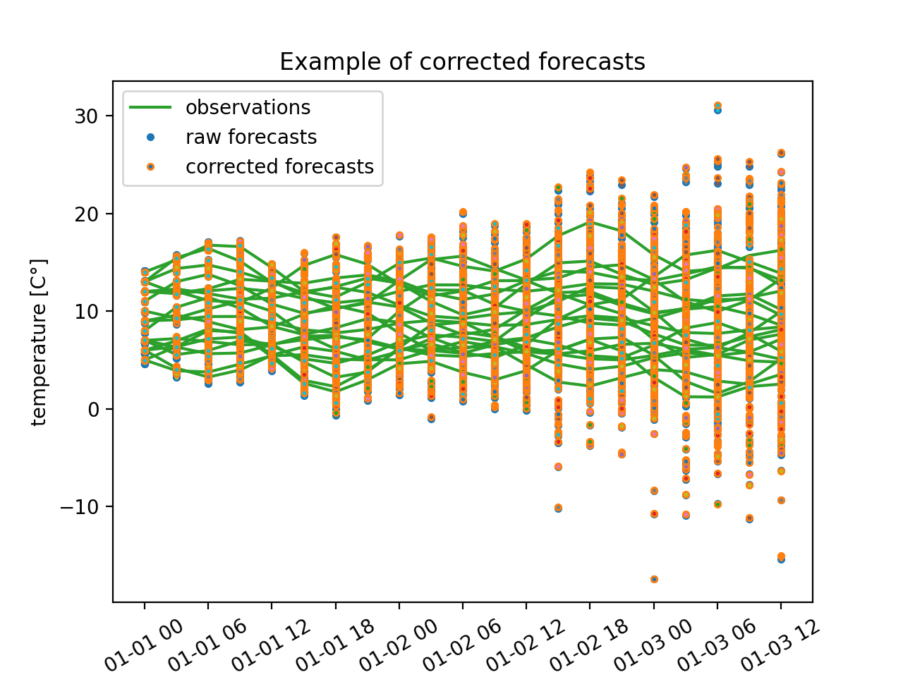
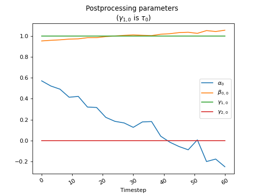
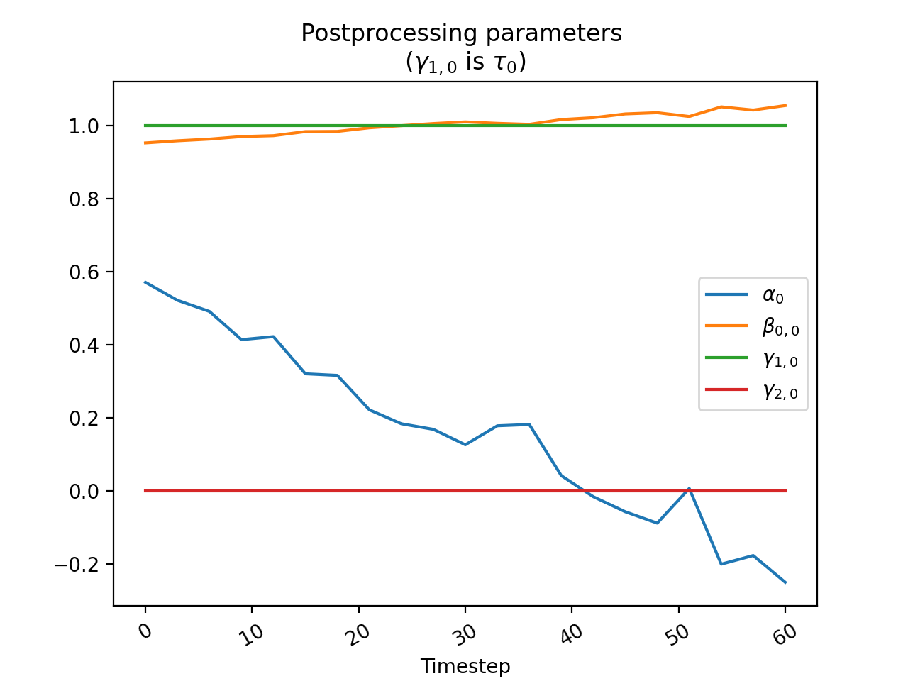
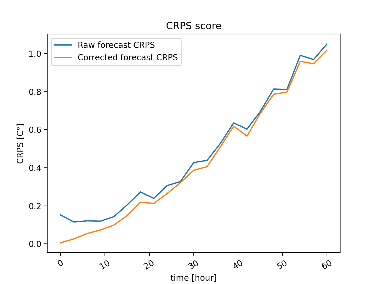
>>> from pp_test.test_data import test_sin
>>> import postprocessors.MBM as MBM
>>> import matplotlib.pyplot as plt
>>>
>>> # Loading random sinusoidal observations and reforecasts
>>> past_observations, reforecasts = test_sin(60., 3., number_of_observation=200)
>>> past_observations.index_shape
(1, 200, 1, 1, 21)
>>> reforecasts.index_shape
(1, 200, 10, 1, 21)
>>>
>>> # Training the postprocessor
>>> postprocessor = MBM.BiasCorrection()
>>> postprocessor.train(past_observations, reforecasts)
>>>
>>> # Loading new random sinusoidal observations and forecasts
>>> observations, forecasts = test_sin(60., 3.)
>>> corrected_forecasts = postprocessor(forecasts)  # Correcting the new forecasts
>>>
>>> # Plotting the forecasts
>>> ax = observations.plot(global_label='observations', color='tab:green')
>>> ax = forecasts.plot(ax=ax, global_label='raw forecasts', mfc=None, mec='tab:blue',
... ls='', marker='o', ms=3.0)
>>> ax = corrected_forecasts.plot(ax=ax, global_label='corrected forecasts', mfc=None,
... mec='tab:orange', ls='', marker='o', ms=3.0)
>>> t = ax.set_ylabel('temperature [C°]')
>>> t = ax.set_xlabel('date')
>>> t = ax.legend()
>>> t = ax.set_title('Example of corrected forecasts')
>>>
>>> # Plotting the bias
>>> ax = postprocessor.plot_parameters()
>>> t = ax.set_title('Postprocessing parameters \n'+r'($\gamma_{1,0}$ is $\tau_{0}$)')
>>>
>>> # Computing the CRPS score
>>> raw_crps = forecasts.CRPS(observations)
>>> corrected_crps = corrected_forecasts.CRPS(observations)
>>>
>>> # Plotting the CRPS score
>>> ax = raw_crps.plot(timestamps=postprocessor.parameters_list[0].timestamps[0, 0],
... global_label='Raw forecast CRPS', color='tab:blue')
>>> ax = corrected_crps.plot(timestamps=postprocessor.parameters_list[0].timestamps[0, 0], ax=ax,
... global_label='Corrected forecast CRPS', color='tab:orange')
>>> t = ax.set_ylabel('CRPS [C°]')
>>> t = ax.set_xlabel('time [hour]')
>>> t = ax.set_title('CRPS score')
>>> t = ax.legend()
>>> plt.show()
- train(observations, predictors, forecast_init_time=None, **kwargs)[source]
Method to train the postprocessor with an observation and predictors training set. Once trained, the postprocessor parameters are stored in the
parameter_list.- Parameters
observations (Data) – A Data object containing the observation training set.
predictors (Data) – A Data object containing the predictors training set. Must be broadcastable with the observations.
forecast_init_time (int or datetime, optional) – The time at which the predictors generation begin (the (re)forecasts initial time). If None, assume that this time is zero (00Z).
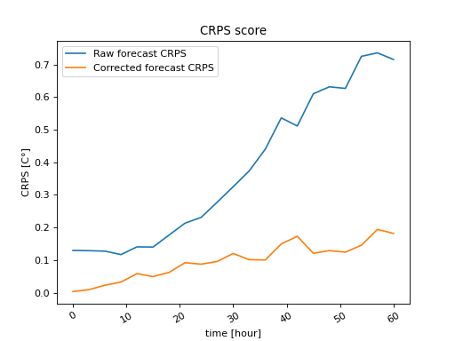
- class postprocessors.MBM.EnsembleAbsCRPSCorrection[source]
Bases:
postprocessors.MBM.EnsembleSpreadScalingCorrectionA postprocessor to correct the ensemble mean and scale the spread of the ensemble. Correct according to the formula:
\[\mathcal{D}^C_{n,m,v} (t) = \alpha_{v} (t) + \sum_{p=1}^P \beta_{p,v} (t) \, \mu^{\rm ens}_{p,n,v} (t) + \left(\gamma_{1,v} (t) + \gamma_{2,v} (t) / \delta_{0, n, v} (t) \right) \, \bar{\mathcal{D}}^{\rm ens}_{0,n,m,v} (t)\]where \(\delta_{0, n, v} (t)\) is the average over the ensemble members of the ensemble members distance (
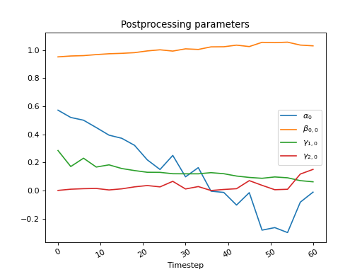
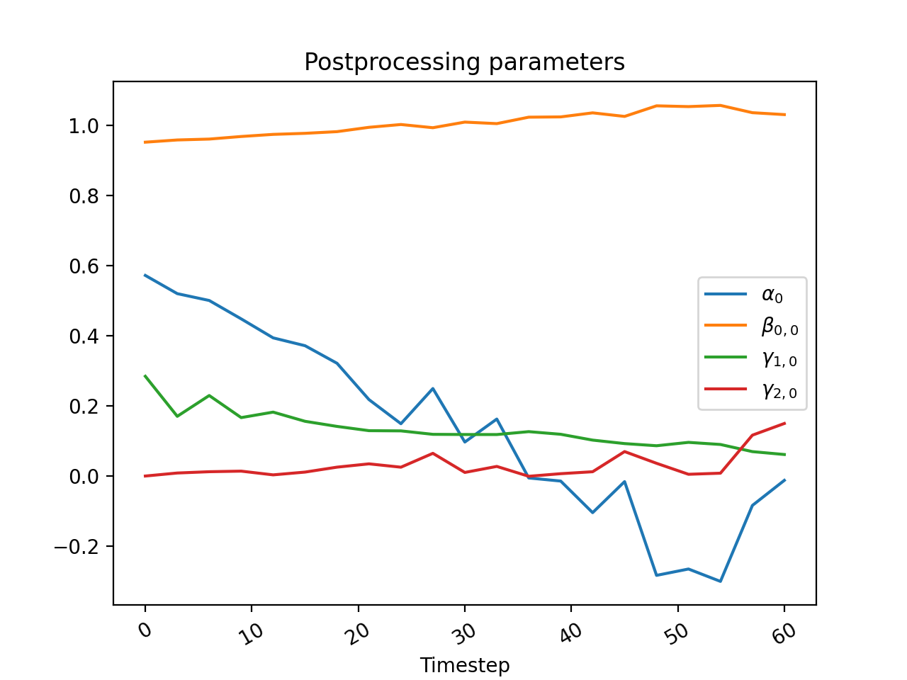
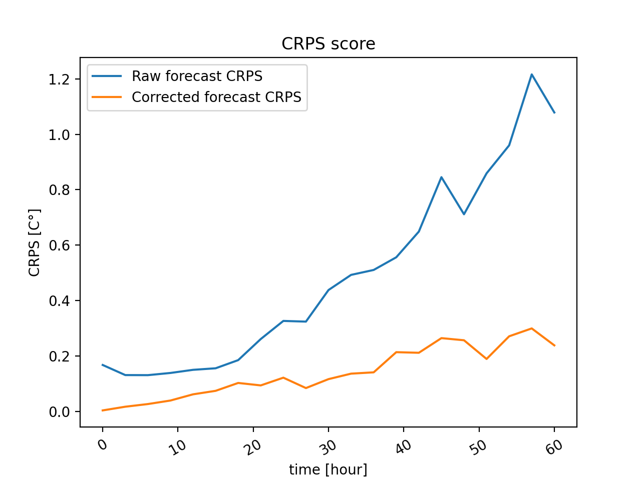
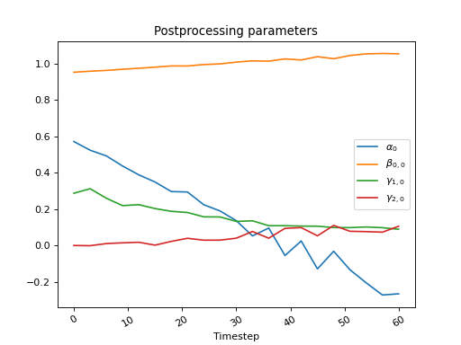
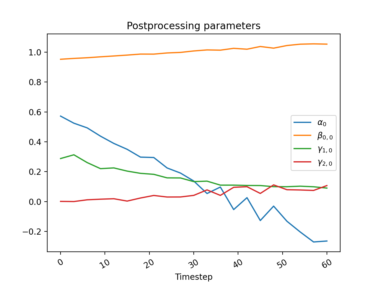
delta). The parameters \(\alpha_{v} (t)\), \(\beta_{v} (t)\), \(\gamma_{1,v} (t)\) and \(\gamma_{2, v} (t)\) are optimized at each lead time to minimize the absolute norm CRPS (Abs_CRPS()) of \(\mathcal{D}^C_{n,m,v} (t)\) with the observations \(\mathcal{O}\). This postprocessor must thus be trained with a training set composed of past ensembles \(\mathcal{D}_{p,n,m,v}\) and observations \(\mathcal{O}\). If needed, the parameters initial conditions for the minimization are constructed using the values given by theEnsembleSpreadScalingCorrection, dependding on the minimizer and options being chosen.The parameters \(\gamma_{1,v} (t)\) and \(\gamma_{2,v} (t)\) control respectively the scaling of the ensemble spread and its nudging toward the climatological variance for the long lead times.
- parameters_list
The list of training parameters \(\alpha_{v} (t)\), \(\beta_{n,v} (t)\), \(\tau_{v} (t)\), as
Dataobjects. This list is empty until the firsttrain()method call.
Examples
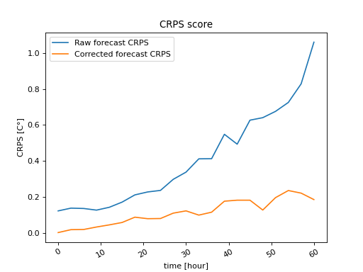
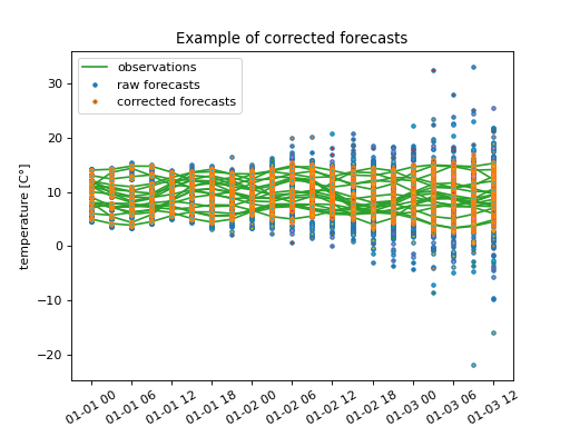
>>> from pp_test.test_data import test_sin
>>> import postprocessors.MBM as MBM
>>> import matplotlib.pyplot as plt
>>>
>>> # Loading random sinusoidal observations and reforecasts
>>> past_observations, reforecasts = test_sin(60., 3., number_of_observation=200)
>>> past_observations.index_shape
(1, 200, 1, 1, 21)
>>> reforecasts.index_shape
(1, 200, 10, 1, 21)
>>>
>>> # Training the postprocessor
>>> postprocessor = MBM.EnsembleAbsCRPSCorrection()
>>> postprocessor.train(past_observations, reforecasts, ntrial=10)
>>>
>>> # Loading new random sinusoidal observations and forecasts
>>> observations, forecasts = test_sin(60., 3.)
>>> corrected_forecasts = postprocessor(forecasts)  # Correcting the new forecasts
>>>
>>> # Plotting the forecasts
>>> ax = observations.plot(global_label='observations', color='tab:green')
>>> ax = forecasts.plot(ax=ax, global_label='raw forecasts', mfc=None, mec='tab:blue',
... ls='', marker='o', ms=3.0)
>>> ax = corrected_forecasts.plot(ax=ax, global_label='corrected forecasts', mfc=None,
... mec='tab:orange', ls='', marker='o', ms=3.0)
>>> t = ax.set_ylabel('temperature [C°]')
>>> t = ax.set_xlabel('date')
>>> t = ax.legend()
>>> t = ax.set_title('Example of corrected forecasts')
>>>
>>> # Plotting the postprocessing parameters
>>> ax = postprocessor.plot_parameters()
>>> t = ax.set_title('Postprocessing parameters')
>>>
>>> # Computing the CRPS score
>>> raw_crps = forecasts.CRPS(observations)
>>> corrected_crps = corrected_forecasts.CRPS(observations)
>>>
>>> # Plotting the CRPS score
>>> ax = raw_crps.plot(timestamps=postprocessor.parameters_list[0].timestamps[0, 0],
... global_label='Raw forecast CRPS', color='tab:blue')
>>> ax = corrected_crps.plot(timestamps=postprocessor.parameters_list[0].timestamps[0, 0], ax=ax,
... global_label='Corrected forecast CRPS', color='tab:orange')
>>> t = ax.set_ylabel('CRPS [C°]')
>>> t = ax.set_xlabel('time [hour]')
>>> t = ax.set_title('CRPS score')
>>> t = ax.legend()
>>> plt.show()


- train(observations, predictors, forecast_init_time=None, num_threads=None, ntrial=1, **kwargs)[source]
Method to train the postprocessor with an observation and predictors training set. Once trained, the postprocessor parameters are stored in the
parameter_list.- Parameters
observations (Data) – A Data object containing the observation training set.
predictors (Data) – A Data object containing the predictors training set. Must be broadcastable with the observations.
forecast_init_time (int or datetime, optional) – The time at which the predictors generation begin (the (re)forecasts initial time). If None, assume that this time is zero (00Z).
num_threads (None or int, optional) – The number of threads used to compute the parameters. One thread computes a chunk of the given grid points and lead times. If None, uses the maximum number of cpu cores available. Default to None.
ntrial (int) – Number of parameters initial conditions to try to find the best solution. Not used if the minimizer being chosen is a global one. Default to 1.
kwargs (dict) – Dictionary of options to pass to the
scipy.optimize.minimize()function.
- class postprocessors.MBM.EnsembleMeanCorrection[source]
Bases:
core.postprocessor.PostProcessorA postprocessor to correct the ensemble mean. Correct according to the formula:
\[\mathcal{D}^C_{n,m,v} (t) = \alpha_{v} (t) + \sum_{p=1}^P \beta_{p,v} (t) \, \mu^{\rm ens}_{p,n,v} (t) + \tau_{v} (t) \bar{\mathcal{D}}^{\rm ens}_{0,n,m,v} (t)\]where \(\alpha_{v} (t) = \left\langle \mathcal{O}_{n,v} (t) - \sum_{p=1}^P \beta_{p,v} (t) \, \mu^{\rm ens}_{p,n,v} (t) \right\rangle_n\) with \(\mathcal{O}_{n,v} (t)\) the observation training set and \(\mu^{\rm ens}_{p,n,v} (t)\) the ensemble mean of the predictors of the training set. \(\bar{\mathcal{D}}^{\rm ens}_{0,n,m,v} (t)\) is the
centered_ensembleof the first predictor. We have also\[\beta_{p,v} (t) = \sum_{p_1=1}^P \, {\rm Cov}^{\rm obs}_{p_1, v} [\bar{\mathcal{O}}^{\rm obs}, \mu^{\rm ens}] (t) \, {\rm Cov}^{\rm obs}_{p_1, p_2, v} [\mu^{\rm ens}, \mu^{\rm ens}] (t)\]where \({\rm Cov}^{\rm obs}_{p_1, v} [\bar{\mathcal{O}}^{\rm obs}, \mu^{\rm ens}]\) is the
ensemble_mean_observational_covariance()with the observation training set \(\mathcal{O}_{n,v} (t)\), and \({\rm Cov}^{\rm obs}_{p_1, p_2, v} [\mu^{\rm ens}, \mu^{\rm ens}]\) is theensemble_mean_observational_self_covariance. Finally, we have \(\tau_{v} (t) = 1\) for all \(v\) and \(t\).- parameters_list
The list of training parameters \(\alpha_{v} (t)\), \(\beta_{n,v} (t)\), \(\tau_{v} (t)\), as
Dataobjects. This list is empty until the firsttrain()method call.
Examples
>>> from pp_test.test_data import test_sin
>>> import postprocessors.MBM as MBM
>>> import matplotlib.pyplot as plt
>>>
>>> # Loading random sinusoidal observations and reforecasts
>>> past_observations, reforecasts = test_sin(60., 3., number_of_observation=200)
>>> past_observations.index_shape
(1, 200, 1, 1, 21)
>>> reforecasts.index_shape
(1, 200, 10, 1, 21)
>>>
>>> # Training the postprocessor
>>> postprocessor = MBM.EnsembleMeanCorrection()
>>> postprocessor.train(past_observations, reforecasts)
>>>
>>> # Loading new random sinusoidal observations and forecasts
>>> observations, forecasts = test_sin(60., 3.)
>>> corrected_forecasts = postprocessor(forecasts)  # Correcting the new forecasts
>>>
>>> # Plotting the forecasts
>>> ax = observations.plot(global_label='observations', color='tab:green')
>>> ax = forecasts.plot(ax=ax, global_label='raw forecasts', mfc=None, mec='tab:blue',
... ls='', marker='o', ms=3.0)
>>> ax = corrected_forecasts.plot(ax=ax, global_label='corrected forecasts', mfc=None,
... mec='tab:orange', ls='', marker='o', ms=3.0)
>>> t = ax.set_ylabel('temperature [C°]')
>>> t = ax.set_xlabel('date')
>>> t = ax.legend()
>>> t = ax.set_title('Example of corrected forecasts')
>>>
>>> # Plotting the postprocessing parameters
>>> ax = postprocessor.plot_parameters()
>>> t = ax.set_title('Postprocessing parameters \n'+r'($\gamma_{1,0}$ is $\tau_{0}$)')
>>>
>>> # Computing the CRPS score
>>> raw_crps = forecasts.CRPS(observations)
>>> corrected_crps = corrected_forecasts.CRPS(observations)
>>>
>>> # Plotting the CRPS score
>>> ax = raw_crps.plot(timestamps=postprocessor.parameters_list[0].timestamps[0, 0],
... global_label='Raw forecast CRPS', color='tab:blue')
>>> ax = corrected_crps.plot(timestamps=postprocessor.parameters_list[0].timestamps[0, 0], ax=ax,
... global_label='Corrected forecast CRPS', color='tab:orange')
>>> t = ax.set_ylabel('CRPS [C°]')
>>> t = ax.set_xlabel('time [hour]')
>>> t = ax.set_title('CRPS score')
>>> t = ax.legend()
>>> plt.show()


- __call__(predictors, predictor_offset=0, proc_time_offset=0, shift_parameters=0, interpolate_offset=None, init_params=None)[source]
Actual postprocessing of new predictors. Return the corrected first predictor.
- Parameters
predictors (Data) – Data object with the predictors to postprocess. The method will get their timestamps and interpolate the parameters for the timestamps that are missing.
predictor_offset (int, optional) – Allow to skip the first predictor_offset values of the given predictors. Default to zero.
proc_time_offset (int, optional) – Indicate at which time in hours the processor start with respect to the start of the forecast. Default to zero.
interpolate_offset (None or int, optional) – Allow to start the interpolation before the first data point, and specify at which time (in hour after the start of the forecast). None to disable. Default to None.
init_params (None or list(int) or list(Data), optional) – Specify the initial parameters of the interpolation if interpolate_offset is set. None to disable. Must be set if interpolate_offset is set. Default to None.
- get_interpolated_parameters(predictors, predictor_offset=0, proc_time_offset=0, interpolate_offset=None, init_params=None)[source]
Method to get the postprocessor parameters interpolated to fix missing timesteps. Assumes that the parameters evolve “smoothly” with the timesteps to fill the gaps.
- Parameters
predictors (Data) – Data object with the predictors to postprocess. The method will get their timestamps and interpolate the parameters for the timestamps that are missing.
predictor_offset (int, optional) – Allow to skip the first predictor_offset values of the given predictors. Default to zero.
proc_time_offset (int, optional) – Indicate at which time in hours the processor start with respect to the start of the forecast. Default to zero.
interpolate_offset (None or int, optional) – Allow to start the interpolation before the first data point, and specify at which time (in hour after the start of the forecast). None to disable. Default to None.
init_params (None or list(int) or list(Data), optional) – Specify the initial parameters of the interpolation if interpolate_offset is set. None to disable. Must be set if interpolate_offset is set. Default to None.
- plot_interpolated_parameters(predictors, proc_kwargs, timestamps=False, variable='all', raw_param_kwargs=None, ax=None, grid_point=None, **kwargs)[source]
Method to plot the postprocessor parameters interpolated to fix missing timesteps obtained by the method
get_interpolated_parameters().- Parameters
predictors (Data) – Data object with the predictors to postprocess. The method will get their timestamps and interpolate the parameters for the timestamps that are missing.
proc_kwargs (dict) – Dictionary of arguments to pass to the
get_interpolated_parameters()method.timestamps (array_like, optional) – Timestamps to pass to the plotting routine. Supersedes the timestamps of the predictors. If False, use the timestamps of the predictors. Default to False.
variable (str, slice, list or int, optional) – Allow to select for which variable to plot the parameters. Default to ‘all’.
raw_param_kwargs (dict) – Dictionary of arguments to pass to the ~.Data.plot method for the raw (not interpolated) parameters.
ax (Axes, optional) – An axes on which to plot.
grid_point (tuple(int, int), optional) – If the data are fields, specifies the parameters of which grid point to plot.
kwargs (dict) – Dictionary of arguments to pass to the ~.Data.plot method for the interpolated parameters.
- Returns
ax – An axes where the parameters were plotted.
- Return type
- train(observations, predictors, forecast_init_time=None, **kwargs)[source]
Method to train the postprocessor with an observation and predictors training set. Once trained, the postprocessor parameters are stored in the
parameter_list.- Parameters
observations (Data) – A Data object containing the observation training set.
predictors (Data) – A Data object containing the predictors training set. Must be broadcastable with the observations.
forecast_init_time (int or datetime, optional) – The time at which the predictors generation begin (the (re)forecasts initial time). If None, assume that this time is zero (00Z).
- class postprocessors.MBM.EnsembleNgrCRPSCorrection[source]
Bases:
postprocessors.MBM.EnsembleAbsCRPSCorrectionA postprocessor to correct the ensemble mean and scale the spread of the ensemble. Correct according to the formula:
\[\mathcal{D}^C_{n,m,v} (t) = \alpha_{v} (t) + \sum_{p=1}^P \beta_{p,v} (t) \, \mu^{\rm ens}_{p,n,v} (t) + \left(\gamma_{1,v} (t) + \gamma_{2,v} (t) / \delta_{0, n, v} (t) \right) \, \bar{\mathcal{D}}^{\rm ens}_{0,n,m,v} (t)\]where \(\delta_{0, n, v} (t)\) is the average over the ensemble members of the ensemble members distance (
delta). The parameters \(\alpha_{v} (t)\), \(\beta_{v} (t)\), \(\gamma_{1,v} (t)\) and \(\gamma_{2,v} (t)\) are optimized at each lead time to minimize Non-homogeneous Gaussian Regression (NGR) CRPS (Abs_Ngr()) of \(\mathcal{D}^C_{n,m,v} (t)\) with the observations \(\mathcal{O}\). This postprocessor must thus be trained with a training set composed of past ensembles \(\mathcal{D}_{p,n,m,v}\) and observations \(\mathcal{O}\). If needed, the parameters initial conditions for the minimization are constructed using the values given by theEnsembleSpreadScalingCorrection, dependding on the minimizer and options being chosen.The parameters \(\gamma_{1,v} (t)\) and \(\gamma_{2,v} (t)\) control respectively the scaling of the ensemble spread and its nudging toward the climatological variance for the long lead times.
- parameters_list
The list of training parameters \(\alpha_{v} (t)\), \(\beta_{n,v} (t)\), \(\tau_{v} (t)\), as
Dataobjects. This list is empty until the firsttrain()method call.
Examples
>>> from pp_test.test_data import test_sin
>>> import postprocessors.MBM as MBM
>>> import matplotlib.pyplot as plt
>>>
>>> # Loading random sinusoidal observations and reforecasts
>>> past_observations, reforecasts = test_sin(60., 3., number_of_observation=200)
>>> past_observations.index_shape
(1, 200, 1, 1, 21)
>>> reforecasts.index_shape
(1, 200, 10, 1, 21)
>>>
>>> # Training the postprocessor
>>> postprocessor = MBM.EnsembleNgrCRPSCorrection()
>>> postprocessor.train(past_observations, reforecasts, ntrial=10)
>>>
>>> # Loading new random sinusoidal observations and forecasts
>>> observations, forecasts = test_sin(60., 3.)
>>> corrected_forecasts = postprocessor(forecasts)  # Correcting the new forecasts
>>>
>>> # Plotting the forecasts
>>> ax = observations.plot(global_label='observations', color='tab:green')
>>> ax = forecasts.plot(ax=ax, global_label='raw forecasts', mfc=None, mec='tab:blue',
... ls='', marker='o', ms=3.0)
>>> ax = corrected_forecasts.plot(ax=ax, global_label='corrected forecasts', mfc=None,
... mec='tab:orange', ls='', marker='o', ms=3.0)
>>> t = ax.set_ylabel('temperature [C°]')
>>> t = ax.set_xlabel('date')
>>> t = ax.legend()
>>> t = ax.set_title('Example of corrected forecasts')
>>>
>>> # Plotting the postprocessing parameters
>>> ax = postprocessor.plot_parameters()
>>> t = ax.set_title('Postprocessing parameters')
>>>
>>> # Computing the CRPS score
>>> raw_crps = forecasts.CRPS(observations)
>>> corrected_crps = corrected_forecasts.CRPS(observations)
>>>
>>> # Plotting the CRPS score
>>> ax = raw_crps.plot(timestamps=postprocessor.parameters_list[0].timestamps[0, 0],
... global_label='Raw forecast CRPS', color='tab:blue')
>>> ax = corrected_crps.plot(timestamps=postprocessor.parameters_list[0].timestamps[0, 0], ax=ax,
... global_label='Corrected forecast CRPS', color='tab:orange')
>>> t = ax.set_ylabel('CRPS [C°]')
>>> t = ax.set_xlabel('time [hour]')
>>> t = ax.set_title('CRPS score')
>>> t = ax.legend()
>>> plt.show()

- class postprocessors.MBM.EnsembleSpreadScalingAbsCRPSCorrection[source]
Bases:
postprocessors.MBM.EnsembleSpreadScalingCorrectionA postprocessor to correct the ensemble mean and scale the spread of the ensemble. Correct according to the formula:
\[\mathcal{D}^C_{n,m,v} (t) = \alpha_{v} (t) + \sum_{p=1}^P \beta_{p,v} (t) \, \mu^{\rm ens}_{p,n,v} (t) + \tau_{v} (t) \bar{\mathcal{D}}^{\rm ens}_{0,n,m,v} (t)\]The parameters \(\alpha_{v} (t)\), \(\beta_{v} (t)\) and \(\tau_{v} (t)\) are optimized at each lead time to minimize the absolute norm CRPS (
Abs_CRPS()) of \(\mathcal{D}^C_{n,m,v} (t)\) with the observations \(\mathcal{O}\). This postprocessor must thus be trained with a training set composed of past ensembles \(\mathcal{D}_{p,n,m,v}\) and observations \(\mathcal{O}\). If needed, the parameters initial conditions for the minimization are constructed using the values given by theEnsembleSpreadScalingCorrection, dependding on the minimizer and options being chosen.- parameters_list
The list of training parameters \(\alpha_{v} (t)\), \(\beta_{n,v} (t)\), \(\tau_{v} (t)\), as
Dataobjects. This list is empty until the firsttrain()method call.
Examples
>>> from pp_test.test_data import test_sin
>>> import postprocessors.MBM as MBM
>>> import matplotlib.pyplot as plt
>>>
>>> # Loading random sinusoidal observations and reforecasts
>>> past_observations, reforecasts = test_sin(60., 3., number_of_observation=200)
>>> past_observations.index_shape
(1, 200, 1, 1, 21)
>>> reforecasts.index_shape
(1, 200, 10, 1, 21)
>>>
>>> # Training the postprocessor
>>> postprocessor = MBM.EnsembleSpreadScalingAbsCRPSCorrection()
>>> postprocessor.train(past_observations, reforecasts, ntrial=10)
>>>
>>> # Loading new random sinusoidal observations and forecasts
>>> observations, forecasts = test_sin(60., 3.)
>>> corrected_forecasts = postprocessor(forecasts)  # Correcting the new forecasts
>>>
>>> # Plotting the forecasts
>>> ax = observations.plot(global_label='observations', color='tab:green')
>>> ax = forecasts.plot(ax=ax, global_label='raw forecasts', mfc=None, mec='tab:blue',
... ls='', marker='o', ms=3.0)
>>> ax = corrected_forecasts.plot(ax=ax, global_label='corrected forecasts', mfc=None,
... mec='tab:orange', ls='', marker='o', ms=3.0)
>>> t = ax.set_ylabel('temperature [C°]')
>>> t = ax.set_xlabel('date')
>>> t = ax.legend()
>>> t = ax.set_title('Example of corrected forecasts')
>>>
>>> # Plotting the postprocessing parameters
>>> ax = postprocessor.plot_parameters()
>>> t = ax.set_title('Postprocessing parameters \n'+r'($\gamma_{1,0}$ is $\tau_{0}$)')
>>>
>>> # Computing the CRPS score
>>> raw_crps = forecasts.CRPS(observations)
>>> corrected_crps = corrected_forecasts.CRPS(observations)
>>>
>>> # Plotting the CRPS score
>>> ax = raw_crps.plot(timestamps=postprocessor.parameters_list[0].timestamps[0, 0],
... global_label='Raw forecast CRPS', color='tab:blue')
>>> ax = corrected_crps.plot(timestamps=postprocessor.parameters_list[0].timestamps[0, 0], ax=ax,
... global_label='Corrected forecast CRPS', color='tab:orange')
>>> t = ax.set_ylabel('CRPS [C°]')
>>> t = ax.set_xlabel('time [hour]')
>>> t = ax.set_title('CRPS score')
>>> t = ax.legend()
>>> plt.show()

- train(observations, predictors, forecast_init_time=None, num_threads=None, ntrial=1, **kwargs)[source]
Method to train the postprocessor with an observation and predictors training set. Once trained, the postprocessor parameters are stored in the
parameter_list.- Parameters
observations (Data) – A Data object containing the observation training set.
predictors (Data) – A Data object containing the predictors training set. Must be broadcastable with the observations.
forecast_init_time (int or datetime, optional) – The time at which the predictors generation begin (the (re)forecasts initial time). If None, assume that this time is zero (00Z).
num_threads (None or int, optional) – The number of threads used to compute the parameters. One thread computes a chunk of the given grid points and lead times. If None, uses the maximum number of cpu cores available. Default to None.
ntrial (int) – Number of parameters initial conditions to try to find the best solution. Not used if the minimizer being chosen is a global one. Default to 1.
kwargs (dict) – Dictionary of options to pass to the
scipy.optimize.minimize()function.
- class postprocessors.MBM.EnsembleSpreadScalingCorrection[source]
Bases:
postprocessors.MBM.EnsembleMeanCorrectionA postprocessor to correct the ensemble mean and scale the spread of the ensemble. Correct according to the formula:
\[\mathcal{D}^C_{n,m,v} (t) = \alpha_{v} (t) + \sum_{p=1}^P \beta_{p,v} (t) \, \mu^{\rm ens}_{p,n,v} (t) + \tau_{v} (t) \bar{\mathcal{D}}^{\rm ens}_{0,n,m,v} (t)\]where \(\alpha_{v} (t) = \left\langle \mathcal{O}_{n,v} (t) - \sum_{p=1}^P \beta_{p,v} (t) \, \mu^{\rm ens}_{p,n,v} (t) \right\rangle_n\) with \(\mathcal{O}_{n,v} (t)\) the observation training set and \(\mu^{\rm ens}_{p,n,v} (t)\) the ensemble mean of the predictors of the training set. \(\bar{\mathcal{D}}^{\rm ens}_{0,n,m,v} (t)\) is the
centered_ensembleof the first predictor. We have also\[\beta_{p,v} (t) = \sum_{p_1=1}^P \, {\rm Cov}^{\rm obs}_{p_1, v} [\bar{\mathcal{O}}^{\rm obs}, \mu^{\rm ens}] (t) \, {\rm Cov}^{\rm obs}_{p_1, p_2, v} [\mu^{\rm ens}, \mu^{\rm ens}] (t)\]where \({\rm Cov}^{\rm obs}_{p_1, v} [\bar{\mathcal{O}}^{\rm obs}, \mu^{\rm ens}]\) is the
ensemble_mean_observational_covariance()with the observation training set \(\mathcal{O}_{n,v} (t)\), and \({\rm Cov}^{\rm obs}_{p_1, p_2, v} [\mu^{\rm ens}, \mu^{\rm ens}]\) is theensemble_mean_observational_self_covariance. Finally, we have\[\tau_{v} (t) = \left\langle \sigma^{\rm{ens}}_{n,v} (t)^2 \right\rangle_n^{-1} \, \left\{ \sigma^{\rm obs}_{v} (t)^2 - \sum_{p=1}^P \, \beta_{p,v} (t) \, {\rm Cov}^{\rm obs}_{p, v} [\bar{\mathcal{O}}^{\rm obs}, \mu^{\rm ens}] (t) \right\}\]for all \(n\), which scales the spread of the ensemble over the lead time \(t\). In this formula, \(\sigma^{\rm{ens}}_{n,v} (t)^2\) and \(\sigma^{\rm obs}_{v} (t)^2\) stands respectively for the ensemble variance (
ensemble_var) and for the observational variance (observational_var) of \(\mathcal{D}\).- parameters_list
The list of training parameters \(\alpha_{v} (t)\), \(\beta_{n,v} (t)\), \(\tau_{v} (t)\), as
Dataobjects. This list is empty until the firsttrain()method call.
Examples
>>> from pp_test.test_data import test_sin
>>> import postprocessors.MBM as MBM
>>> import matplotlib.pyplot as plt
>>>
>>> # Loading random sinusoidal observations and reforecasts
>>> past_observations, reforecasts = test_sin(60., 3., number_of_observation=200)
>>> past_observations.index_shape
(1, 200, 1, 1, 21)
>>> reforecasts.index_shape
(1, 200, 10, 1, 21)
>>>
>>> # Training the postprocessor
>>> postprocessor = MBM.EnsembleSpreadScalingCorrection()
>>> postprocessor.train(past_observations, reforecasts)
>>>
>>> # Loading new random sinusoidal observations and forecasts
>>> observations, forecasts = test_sin(60., 3.)
>>> corrected_forecasts = postprocessor(forecasts)  # Correcting the new forecasts
>>>
>>> # Plotting the forecasts
>>> ax = observations.plot(global_label='observations', color='tab:green')
>>> ax = forecasts.plot(ax=ax, global_label='raw forecasts', mfc=None, mec='tab:blue',
... ls='', marker='o', ms=3.0)
>>> ax = corrected_forecasts.plot(ax=ax, global_label='corrected forecasts', mfc=None,
... mec='tab:orange', ls='', marker='o', ms=3.0)
>>> t = ax.set_ylabel('temperature [C°]')
>>> t = ax.set_xlabel('date')
>>> t = ax.legend()
>>> t = ax.set_title('Example of corrected forecasts')
>>>
>>> # Plotting the postprocessing parameters
>>> ax = postprocessor.plot_parameters()
>>> t = ax.set_title('Postprocessing parameters \n'+r'($\gamma_{1,0}$ is $\tau_{0}$)')
>>>
>>> # Computing the CRPS score
>>> raw_crps = forecasts.CRPS(observations)
>>> corrected_crps = corrected_forecasts.CRPS(observations)
>>>
>>> # Plotting the CRPS score
>>> ax = raw_crps.plot(timestamps=postprocessor.parameters_list[0].timestamps[0, 0],
... global_label='Raw forecast CRPS', color='tab:blue')
>>> ax = corrected_crps.plot(timestamps=postprocessor.parameters_list[0].timestamps[0, 0], ax=ax,
... global_label='Corrected forecast CRPS', color='tab:orange')
>>> t = ax.set_ylabel('CRPS [C°]')
>>> t = ax.set_xlabel('time [hour]')
>>> t = ax.set_title('CRPS score')
>>> t = ax.legend()
>>> plt.show()


- train(observations, predictors, forecast_init_time=None, **kwargs)[source]
Method to train the postprocessor with an observation and predictors training set. Once trained, the postprocessor parameters are stored in the
parameter_list.- Parameters
observations (Data) – A Data object containing the observation training set.
predictors (Data) – A Data object containing the predictors training set. Must be broadcastable with the observations.
forecast_init_time (int or datetime, optional) – The time at which the predictors generation begin (the (re)forecasts initial time). If None, assume that this time is zero (00Z).
- class postprocessors.MBM.EnsembleSpreadScalingNgrCRPSCorrection[source]
Bases:
postprocessors.MBM.EnsembleSpreadScalingAbsCRPSCorrectionA postprocessor to correct the ensemble mean and scale the spread of the ensemble. Correct according to the formula:
\[\mathcal{D}^C_{n,m,v} (t) = \alpha_{v} (t) + \sum_{p=1}^P \beta_{p,v} (t) \, \mu^{\rm ens}_{p,n,v} (t) + \tau_{v} (t) \bar{\mathcal{D}}^{\rm ens}_{0,n,m,v} (t)\]The parameters \(\alpha_{v} (t)\), \(\beta_{v} (t)\) and \(\tau_{v} (t)\) are optimized at each lead time to minimize the Non-homogeneous Gaussian Regression (NGR) CRPS (
Abs_Ngr()) of \(\mathcal{D}^C_{n,m,v} (t)\) with the observations \(\mathcal{O}\). This postprocessor must thus be trained with a training set composed of past ensembles \(\mathcal{D}_{p,n,m,v}\) and observations \(\mathcal{O}\). If needed, the parameters initial conditions for the minimization are constructed using the values given by theEnsembleSpreadScalingCorrection, dependding on the minimizer and options being chosen.- parameters_list
The list of training parameters \(\alpha_{v} (t)\), \(\beta_{n,v} (t)\), \(\tau_{v} (t)\), as
Dataobjects. This list is empty until the firsttrain()method call.
Examples
>>> from pp_test.test_data import test_sin
>>> import postprocessors.MBM as MBM
>>> import matplotlib.pyplot as plt
>>>
>>> # Loading random sinusoidal observations and reforecasts
>>> past_observations, reforecasts = test_sin(60., 3., number_of_observation=200)
>>> past_observations.index_shape
(1, 200, 1, 1, 21)
>>> reforecasts.index_shape
(1, 200, 10, 1, 21)
>>>
>>> # Training the postprocessor
>>> postprocessor = MBM.EnsembleSpreadScalingNgrCRPSCorrection()
>>> postprocessor.train(past_observations, reforecasts, ntrial=10)
>>>
>>> # Loading new random sinusoidal observations and forecasts
>>> observations, forecasts = test_sin(60., 3.)
>>> corrected_forecasts = postprocessor(forecasts)  # Correcting the new forecasts
>>>
>>> # Plotting the forecasts
>>> ax = observations.plot(global_label='observations', color='tab:green')
>>> ax = forecasts.plot(ax=ax, global_label='raw forecasts', mfc=None, mec='tab:blue',
... ls='', marker='o', ms=3.0)
>>> ax = corrected_forecasts.plot(ax=ax, global_label='corrected forecasts', mfc=None,
... mec='tab:orange', ls='', marker='o', ms=3.0)
>>> t = ax.set_ylabel('temperature [C°]')
>>> t = ax.set_xlabel('date')
>>> t = ax.legend()
>>> t = ax.set_title('Example of corrected forecasts')
>>>
>>> # Plotting the postprocessing parameters
>>> ax = postprocessor.plot_parameters()
>>> t = ax.set_title('Postprocessing parameters \n'+r'($\gamma_{1,0}$ is $\tau_{0}$)')
>>>
>>> # Computing the CRPS score
>>> raw_crps = forecasts.CRPS(observations)
>>> corrected_crps = corrected_forecasts.CRPS(observations)
>>>
>>> # Plotting the CRPS score
>>> ax = raw_crps.plot(timestamps=postprocessor.parameters_list[0].timestamps[0, 0],
... global_label='Raw forecast CRPS', color='tab:blue')
>>> ax = corrected_crps.plot(timestamps=postprocessor.parameters_list[0].timestamps[0, 0], ax=ax,
... global_label='Corrected forecast CRPS', color='tab:orange')
>>> t = ax.set_ylabel('CRPS [C°]')
>>> t = ax.set_xlabel('time [hour]')
>>> t = ax.set_title('CRPS score')
>>> t = ax.legend()
>>> plt.show()


