Example of gridded forecasts postprocessing
In this example, using Pythie, we postprocess the 2 metre temperature forecasts at a station. We postprocess it with the 2 metre temperature itself, the maximum 2 metre temperature in the last 6 hours and the soil temperature as predictors.
We use the ERA5 reanalysis over a large area in Europe from 1997 to 2016 as gridded observations. These reanalysis have been downloaded from the Copernicus Data Store and converted to the NetCDF file format.
The postprocessing is done by making a regression, at each grid point and lead time, between the gridded reforecasts and the gridded reanalysis (considered as observation). For verification, the result of this regression is then applied on the reforecasts themselves (the training set).
The reforecasts files have been download from ECMWF and converted to NetCDF files.
Note: In the following example, we drop the initial conditions of the reforecasts because one of the maximum 2 meter temperature is not defined at this lead time ! As a result, we do not postprocess the lead time 0.
Gridded reforecast data source
Source: www.ecmwf.int
Creative Commons Attribution 4.0 International (CC BY 4.0) Copyright © 2021 European Centre for Medium-Range Weather Forecasts (ECMWF). See the attached ECMWF_LICENSE.txt file included with the data for more details.
Copernicus ERA5 gridded reanalysis data source
Source: https://cds.climate.copernicus.eu/
Copyright © 2021 European Union. Generated using Copernicus Climate Change Service information 2021.
Hersbach et al. (2018): ERA5 hourly data on single levels from 1979 to present. Copernicus Climate Change Service (C3S) Climate Data Store (CDS). (Accessed on < 21-04-2021 >), doi:10.24381/cds.adbb2d47.
See the attached COPERNICUS_LICENSE.txt file included with the data for more details.
Preliminaries
Setting the path
import sys, os
sys.path.extend([os.path.abspath('../../../../')])
os.chdir('../../../../')
Importing external modules
import iris
import iris.pandas as ipd
import iris.plot as iplt
import iris.quickplot as qplt
import cartopy
import cartopy.crs as ccrs
import cartopy.feature as cfeature
import datetime
import cftime
import matplotlib.pyplot as plt
import matplotlib.animation as animation
from matplotlib import cm
import numpy as np
from IPython.display import HTML
from matplotlib import rc
rc('font',**{'family':'serif','sans-serif':['Times'],'size':16})
%matplotlib inline
Importing internal modules
from core.data import Data
import postprocessors.MBM as MBM
Setting some parameters
# Date of the forecast
date = "01-02"
# Year to correct
year = 2017
# Number of reforecasts
years_back = 20
# Parameter of the analysis (to be postprocessed)
param = '2t'
# Parameters of the predictors
params = ['2t', 'mx2t6', 'stl1']
# Time units used in the NetCDF input files
time_units = 'hours since 1900-01-01 00:00:00.0'
# Locaction of the data
data_folder = './data/europa_grid/'
Defining some functions to extract the time coordinates from Iris cubes
def get_cubes_time_index(cubes):
# assumes all the cube in cubes have the same timestamps
a = ipd.as_data_frame(cubes[0][:, 0, 0])
return a.index
def get_cubes_time(cubes, units=None, year=None):
time_index = get_cubes_time_index(cubes)
if year is not None:
convert_time = lambda t: datetime.datetime(year, t.month, t.day, t.hour)
else:
convert_time = lambda t: datetime.datetime(t.year, t.month, t.day, t.hour)
time = np.array(list(map(convert_time, time_index.values)), dtype=object)
if units is not None:
cf_time = cftime.date2num(time, units=units)
return time, cf_time
else:
return time, None
Defining some plotting functions
def plot_cube(cube, t, v, ax=None, quick=True):
if ax is None:
map_proj = ccrs.PlateCarree()
plt.figure(figsize=(15, 10))
ax = plt.axes(projection=map_proj)
extent = [-20, 20, 30, 70]
ax.gridlines()
ax.coastlines(resolution='50m')
ax.add_feature(cartopy.feature.BORDERS)
if quick:
qplt.contourf(cube[t, :, :], v, axes=ax, cmap=cm.get_cmap('bwr'))
else:
iplt.contourf(cube[t, :, :], v, axes=ax, cmap=cm.get_cmap('bwr'))
ax.set_extent(extent)
return ax
def plot_quant(quant, labels, timestamps, grid_point):
fig = plt.figure(figsize=(15, 10))
ax = fig.gca()
first = True
for c, lab in zip(quant, labels):
if first:
c.plot(ax=ax, global_label=lab, timestamps=timestamps, lw=3., ls="--", grid_point=grid_point)
first = False
else:
c.plot(ax=ax, global_label=lab, timestamps=timestamps, grid_point=grid_point)
ax.legend()
return ax
Loading and creating the Data objects
This section shows how to load Data objects from NetCDF files using Iris
First we load the reforecasts
# For each year in the past:
for y in range(year-years_back, year):
# We load the reforecasts with Iris
reforecast_cubes = iris.load(data_folder+'reforecasts_'+'-'.join(params)+'_'+str(y)+'-'+date+'.nc')
# If it is the first year, then:
if y == year-years_back:
# We create one list per predictors:
reforecasts_list = list()
for i in range(len(reforecast_cubes)):
reforecasts_list.append(list())
# And a list for the timestamps:
times = list()
# We extract the time:
time, t = get_cubes_time(reforecast_cubes, time_units)
times.append(time[1:, ...])
# We create a Numpy array for each variable from the Iris cube
for i, cube in enumerate(reforecast_cubes):
# (we have to swap the time and ensemble member axis and add 2 dummy axis at the beginning
# to fit the Data object specs)
data = np.array(cube.data[1:, ...]).swapaxes(0, 1)[np.newaxis, np.newaxis, ...]
# (and also add the dummy 'variable' axis)
data = np.expand_dims(data, 3)
reforecasts_list[i].append(data)
# Now that the data have been loaded into convenient Numpy arrays, we can create the Data object:
# First create one Data object per predictor
reforecasts_data_list = list()
for reforecast in reforecasts_list:
reforecasts_data_list.append(Data(np.concatenate(reforecast, axis=1), timestamps=times))
# saving the first predictor (the variable itself) for latter
reforecast_data_1st_predictor = reforecasts_data_list[0].copy()
# (Deleting data not needed anymore to save RAM space)
del reforecast_cubes, reforecasts_list
# Then loading all the predictors into one single Data object
reforecasts_data = reforecasts_data_list[0].copy()
for reforecast in reforecasts_data_list[1:]:
reforecasts_data.append_predictors(reforecast)
# (Deleting data not needed anymore to save RAM space)
del reforecasts_data_list
Then we load the analysis
# Same as previously but fo only one variable
analysis = list()
times = list()
for y in range(year-years_back, year):
analysis_cube = iris.load(data_folder+'analysis_'+param+'_'+str(y)+'-'+date+'.nc')
time, t = get_cubes_time(analysis_cube, time_units)
times.append(time[1:, ...])
data = np.array(analysis_cube[0].data[1:, ...])[np.newaxis, np.newaxis, np.newaxis, np.newaxis, ...]
analysis.append(data)
analysis_data = Data(np.concatenate(analysis, axis=1), timestamps=times)
del analysis
Training the PostProcessors
In this section, we train the various different postprocessors of the Member-By-Member MBM module with the data previously loaded
# List to hold the trained PostProcessors
postprocessors = list()
proc_labels = list()
Simple bias correction
ebc = MBM.BiasCorrection()
ebc.train(analysis_data, reforecasts_data)
postprocessors.append(ebc)
proc_labels.append('Bias correction')
Ensemble Mean correction
emc = MBM.EnsembleMeanCorrection()
emc.train(analysis_data, reforecasts_data)
postprocessors.append(emc)
proc_labels.append('Ensemble Mean correction')
Ensemble Spread Scaling correction
essc = MBM.EnsembleSpreadScalingCorrection()
essc.train(analysis_data, reforecasts_data)
postprocessors.append(essc)
proc_labels.append('Ensemble Spread Scaling correction')
Ensemble Spread Scaling correction with Absolute norm CRPS minimization
essacc = MBM.EnsembleSpreadScalingAbsCRPSCorrection()
essacc.train(analysis_data, reforecasts_data, ntrial=1)
postprocessors.append(essacc)
proc_labels.append('Ensemble Spread Scaling Abs. CRPS min. correction')
Ensemble Spread Scaling correction + Climatology nudging with Absolute norm CRPS minimization
eacc = MBM.EnsembleAbsCRPSCorrection()
eacc.train(analysis_data, reforecasts_data, ntrial=1)
postprocessors.append(eacc)
proc_labels.append('Ensemble Spread Scaling + Clim. Nudging Abs. CRPS min. correction')
Ensemble Spread Scaling correction + Climatology nudging with Ngr CRPS minimization
encc = MBM.EnsembleNgrCRPSCorrection()
encc.train(analysis_data, reforecasts_data, ntrial=1)
postprocessors.append(encc)
proc_labels.append('Ensemble Spread Scaling + Clim. Nudging Ngr CRPS min. correction')
Verification
Here we are going to postprocess the reforecasts themselves to see how well they perform:
# List to store the experiment names
exp_results = list()
exp_results.append(reforecast_data_1st_predictor)
exp_labels = list()
exp_labels.append('Raw forecasts')
timestamps = np.array(range(reforecast_data_1st_predictor.number_of_time_steps))
for label, postprocessor in zip(proc_labels, postprocessors):
exp_results.append(postprocessor(reforecasts_data))
exp_labels.append(label)
Computing scores
Computing the bias
# List to store the CRPS Data object
bias = list()
for label, result in zip(exp_labels, exp_results):
bias.append(result.bias(analysis_data))
Computing the ensemble mean RMSE
# List to store the CRPS Data object
rmse = list()
for label, result in zip(exp_labels, exp_results):
rmse.append(result.ensemble_mean_RMSE(analysis_data))
Computing the CRPS
# List to store the CRPS Data object
crps = list()
for label, result in zip(exp_labels, exp_results):
crps.append(result.CRPS(analysis_data))
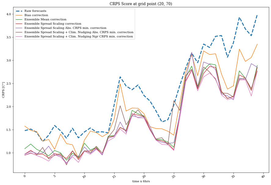
Plotting the scores
Plots at a grid point
grid_point=(20,70)
ax = plot_quant(crps, exp_labels, timestamps, grid_point=grid_point)
ax.set_title('CRPS Score at grid point '+str(grid_point))
ax.set_ylabel('CRPS [C°]')
ax.set_xlabel('time x 6hrs');
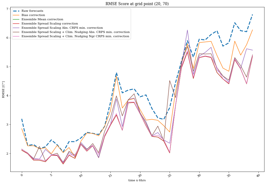
ax = plot_quant(rmse, exp_labels, timestamps, grid_point=grid_point)
ax.set_title('RMSE Score at grid point '+str(grid_point))
ax.set_ylabel('RMSE [C°]')
ax.set_xlabel('time x 6hrs');
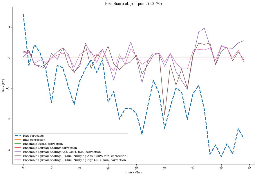
ax = plot_quant(bias, exp_labels, timestamps, grid_point=grid_point)
ax.set_title('Bias Score at grid point '+str(grid_point))
ax.set_ylabel('Bias [C°]')
ax.set_xlabel('time x 6hrs');
Plotting scores as fields
Creating Iris CubeLists to store the scores:
crps_cubes = iris.cube.CubeList()
bias_cubes = iris.cube.CubeList()
rmse_cubes = iris.cube.CubeList()
Creating the bias cubes
for score in bias:
# Creating a cube by recycling the analysis one
bias_cube = analysis_cube[0].copy()
# And replacing the data inside by the score
bias_cube.data[1:, :, :] = np.squeeze(score.data)
bias_cubes.append(bias_cube[1:])
for score in rmse:
# Creating a cube by recycling the analysis one
rmse_cube = analysis_cube[0].copy()
# And replacing the data inside by the score
rmse_cube.data[1:, :, :] = np.squeeze(score.data)
rmse_cubes.append(rmse_cube[1:])
for score in crps:
# Creating a cube by recycling the analysis one
crps_cube = analysis_cube[0].copy()
# And replacing the data inside by the score
crps_cube.data[1:, :, :] = np.squeeze(score.data)
crps_cubes.append(crps_cube[1:])
# Countour plot levels in Celsius
t2m_range = np.arange(-4.,4.,0.25)
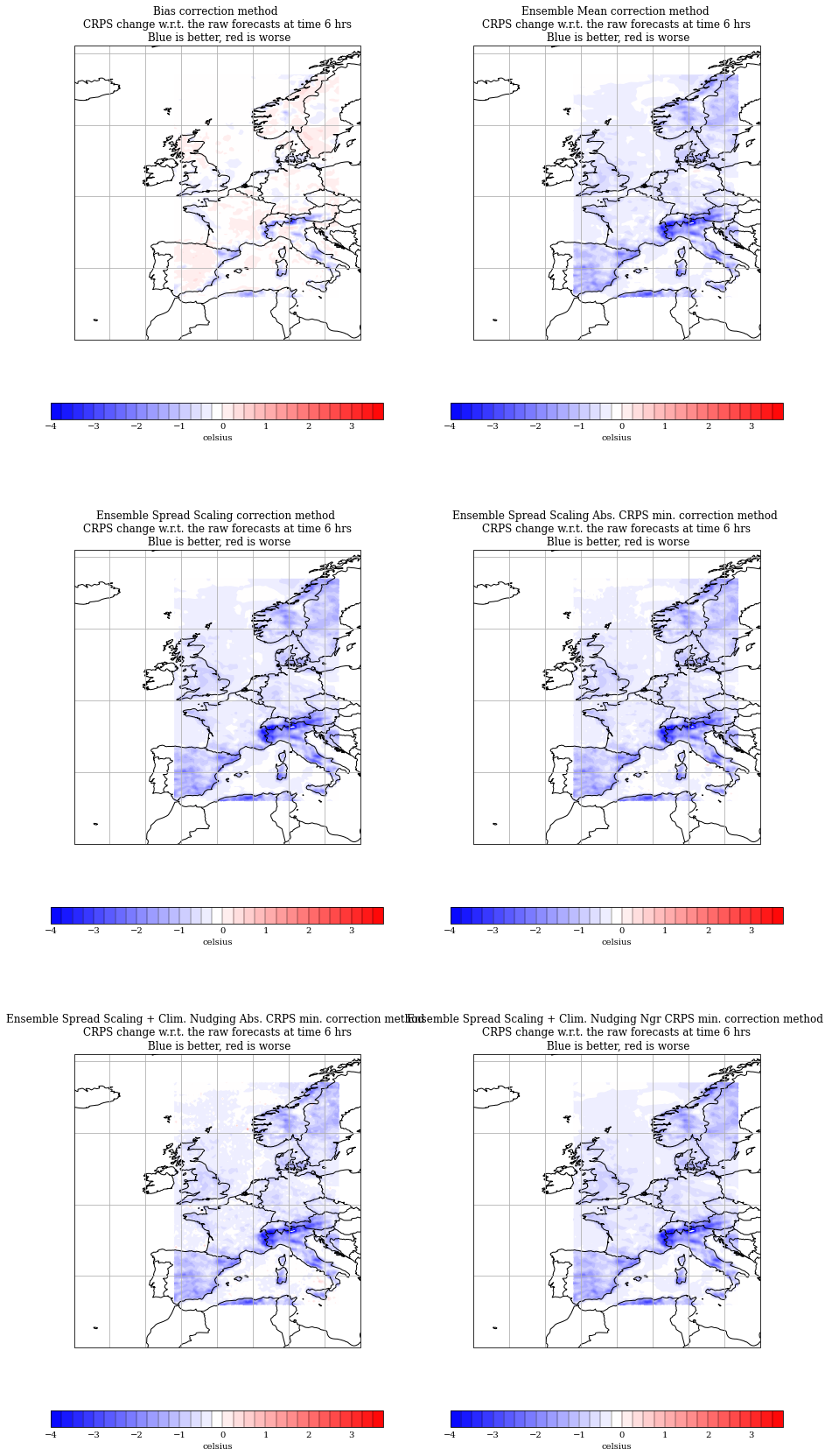
Plot of the CRPS improvement
frames = crps_cubes[0].shape[0]
map_proj = ccrs.PlateCarree()
ns = len(rmse_cubes)-1
nr = int(np.ceil(ns / 2))
axls = list()
fig=plt.figure(figsize=(15, 10 * nr))
t = 0
for i in range(ns):
plt.subplot(nr, 2, i+1, projection=map_proj)
ax = plt.gca()
axls.append(ax)
plot_cube(crps_cubes[i+1]-crps_cubes[0], t, t2m_range, ax=ax)
ax.set_title(exp_labels[i+1]+' method \nCRPS change w.r.t. the raw forecasts at time '+str((t+1)*6)+' hrs\n Blue is better, red is worse')
def update(t):
imlist = list()
for i in range(ns):
ax = axls[i]
ax.clear()
plot_cube(crps_cubes[i+1]-crps_cubes[0], t, t2m_range, ax=ax, quick=False)
ax.set_title(exp_labels[i+1]+' method \nCRPS change w.r.t. the raw forecasts at time '+str((t+1)*6)+' hrs\n Blue is better, red is worse')
imlist.append(ax._gci())
return imlist
crps_anim = animation.FuncAnimation(fig, update, frames=frames, interval=250, blit=False)
Making a video to show the CRPS evolution over the lead time
HTML(crps_anim.to_html5_video())
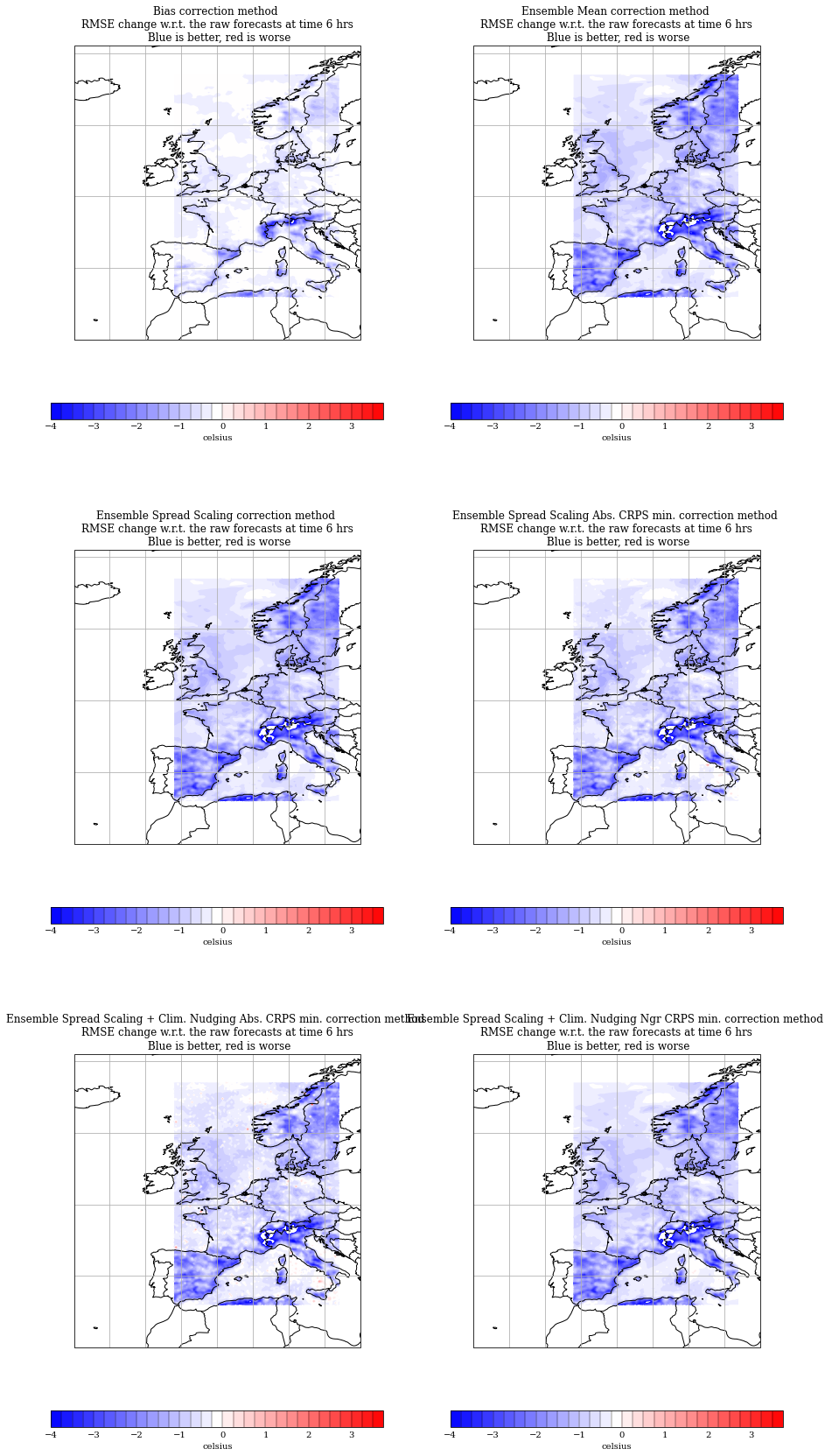
Plot of the RMSE improvement
frames = bias_cubes[0].shape[0]
map_proj = ccrs.PlateCarree()
ns = len(rmse_cubes)-1
nr = int(np.ceil(ns / 2))
axls = list()
fig=plt.figure(figsize=(15, 10 * nr))
t = 0
for i in range(ns):
plt.subplot(nr, 2, i+1, projection=map_proj)
ax = plt.gca()
axls.append(ax)
plot_cube(rmse_cubes[i+1]-rmse_cubes[0], t, t2m_range, ax=ax)
ax.set_title(exp_labels[i+1]+' method \nRMSE change w.r.t. the raw forecasts at time '+str((t+1)*6)+' hrs\n Blue is better, red is worse')
def update(t):
imlist = list()
for i in range(ns):
ax = axls[i]
ax.clear()
plot_cube(rmse_cubes[i+1]-rmse_cubes[0], t, t2m_range, ax=ax, quick=False)
ax.set_title(exp_labels[i+1]+' method \nRMSE change w.r.t. the raw forecasts at time '+str((t+1)*6)+' hrs\n Blue is better, red is worse')
imlist.append(ax._gci())
return imlist
rmse_anim = animation.FuncAnimation(fig, update, frames=frames, interval=250, blit=False)
Making a video to show the RMSE evolution over the lead time
HTML(rmse_anim.to_html5_video())
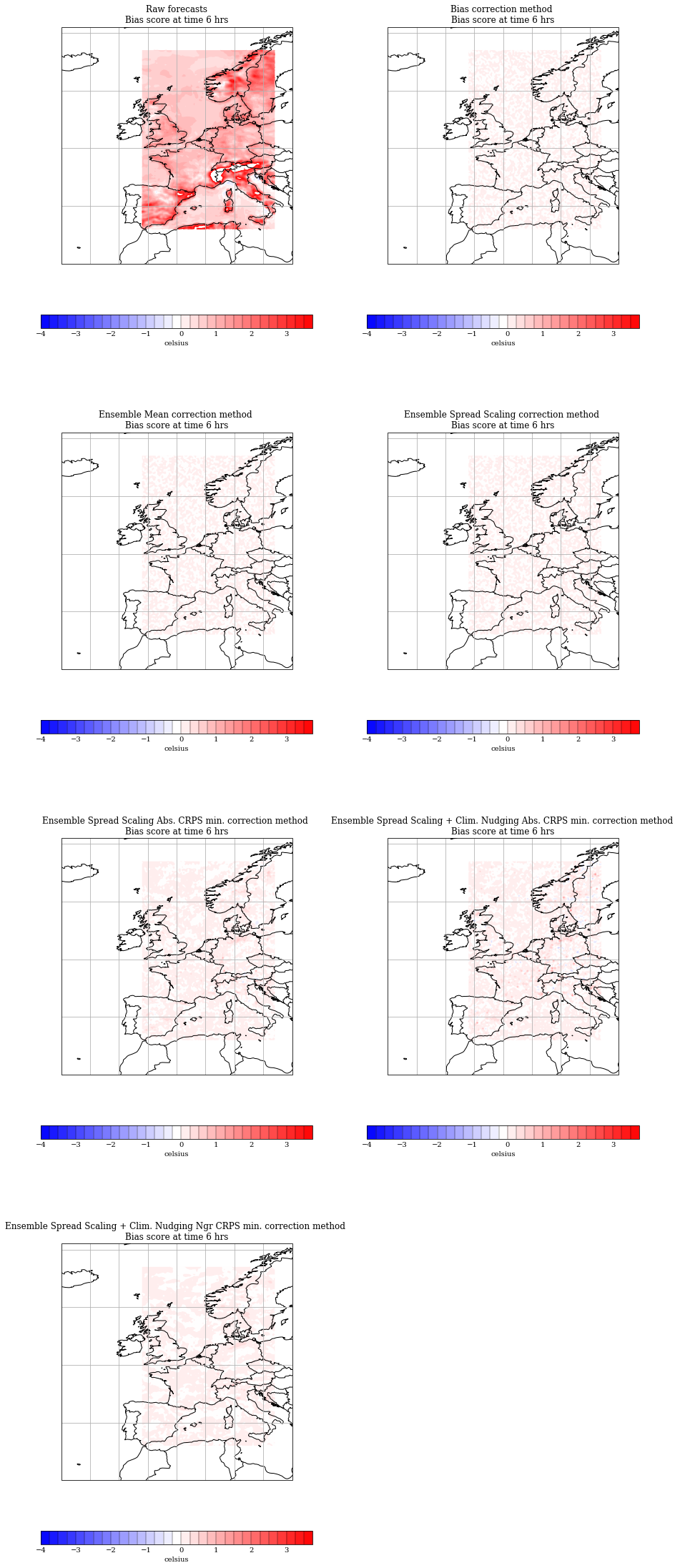
Plot of the bias
frames = bias_cubes[0].shape[0]
map_proj = ccrs.PlateCarree()
ns = len(bias_cubes)
nr = int(np.ceil(ns / 2))
axls = list()
fig=plt.figure(figsize=(15, 10 * nr))
t = 0
for i in range(ns):
plt.subplot(nr, 2, i+1, projection=map_proj)
ax = plt.gca()
axls.append(ax)
plot_cube(bias_cubes[i], t, t2m_range, ax=ax)
if i >= 1:
ax.set_title(exp_labels[i]+' method \nBias score at time '+str((t+1)*6)+' hrs')
else:
ax.set_title(exp_labels[i]+'\nBias score at time '+str((t+1)*6)+' hrs')
def update(t):
imlist = list()
for i in range(ns):
ax = axls[i]
ax.clear()
plot_cube(bias_cubes[i], t, t2m_range, ax=ax, quick=False)
if i >= 1:
ax.set_title(exp_labels[i]+' method \nBias score at time '+str((t+1)*6)+' hrs')
else:
ax.set_title(exp_labels[i]+'\nBias score at time '+str((t+1)*6)+' hrs')
imlist.append(ax._gci())
return imlist
bias_anim = animation.FuncAnimation(fig, update, frames=frames, interval=250, blit=False)
Making a video to show the bias evolution over the lead time
HTML(bias_anim.to_html5_video())